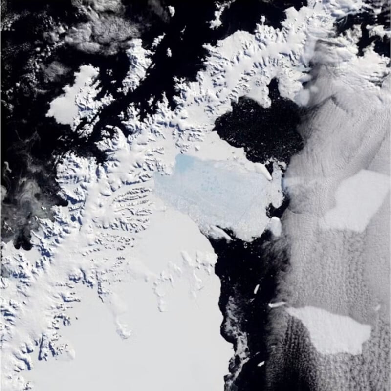
The Larsen Ice Shelf in Antarctica has been breaking up for decades, but the collapse of Larsen B in 2002 was particularly dramatic. After being stable for at least 10,000 years, much of the shelf broke up, with planet-wide consequences.
Large-scale changes in Antarctica have been widely studied and published, but contextualizing and analyzing how changing conditions in Antarctica affect the rest of the world has been challenging. To combat this, scientists used film stills from the 1960s to help understand how collapsing Antarctic ice sheets have affected global sea levels.
In a research paper published in Nature, Ryan North and Timothy T. Barrows examine historical film photographs of Antarctica dating back to the 1940s and apply a sophisticated modern analytical technique called structure-from-motion photogrammetry (SfM). The researchers say: “This technique creates digital elevation models (DEMs) by constructing 3D point clouds of matching features in overlapping photographs without the need for the original position or orientation of the camera.
As North and Barrows explain in an article about ConversationAn accurate understanding of the past is essential to predicting the future.
“To accurately predict how Antarctic ice sheets will respond to future climate change, it is important to understand how they have responded in the past,” the researchers write.
A significant challenge is that Antarctica is remote and acquiring good data there is prohibitively expensive. While satellites are excellent for collecting data over much of the Earth’s surface, the Antarctic Peninsula is shrouded in clouds for most of the year. As a result, observations of the area are irregular and short-lived.
However, US Navy cartographers captured more than 300,000 aerial photographs of Antarctica, all of which are freely available at the Polar Geospatial Center at the University of Minnesota, as part of an extensive mapping of the continent between 1946 and 2000.
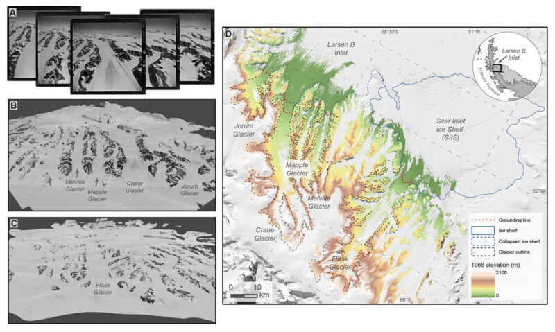
Large-format film photographs are extremely high-resolution, so North and Barrows used SfM photogrammetry on 871 specific photographs from 1968 to create historical data for the Larsen B region.
The selected photographs were captured on large-format 9×9 grayscale film on December 21, 23, and 27, 1968. The film was then scanned at 1,000 DPI by the United States Geological Survey (USGS). 503 of the 867 photographs were used to construct data for the Jorum, Crane, Mapple, and Melville Glaciers, while more than 360 were used to determine the elevation of the Flask Glacier. The images were also manually fine-tuned to reduce errors in the photogrammetric process, including changes in cropping, exposure, contrast and brightness.
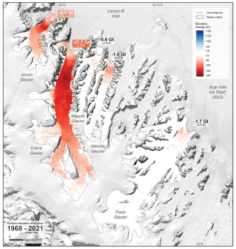
“We use historical DEMs to accurately measure the net elevation change of Larsen B tributary glaciers (Jorum, Crane, Mapple, Melville, and Flask) between 1968 and 2021. We also calculate elevation differences for the same glaciers between 1968 and 2001… Using the exact elevation differences we provide new estimates of the mass balance and sea level contribution over 53 years and discuss these measurements in the context of the existing pre-collapse and post-collapse literature,” they explain.
As a result of their research, the pair determined the exact changes in elevation in individual areas of Larsen B, detailing the exceptionally small changes over the decades that ultimately led to the collapse of the ice shelf. They found that after the collapse of Larsen B in 2002, the glaciers lost a staggering 35 billion tons of land ice. The largest glacier alone lost 28 billion tons, causing the Earth’s sea level to rise by about 0.1 millimeter.
“That doesn’t sound like much,” admit the researchers. “But it’s the result of one iceberg from one event. In other words, it’s the same as if every person on Earth tipped a liter bottle of water every day for 10 years.”
North and Barrow call the historic archive of aerial film footage “an invaluable resource waiting to be tapped” and say the same process they used for this investigation can be used to analyze other ice shelves or glaciers, penguin colonies, vegetation expansion or even direct human activity.
Antarctic ice shelves and glaciers will continue to evolve as climate change accelerates and impacts the rest of the planet. Of course, one of the most critical steps to solving a problem requires understanding the problem itself.
Image credits: Unless otherwise noted, photographs in this article are courtesy of the Polar Geospatial Center and the United States Geological Survey. The research in question is “High-resolution elevation models of Larsen B glaciers derived from 1960s imagery” written by Ryan North and Timothy T. Barrows.